
PyTorch Distributions (Continuous)
Optional Lab: Python, NumPy and Vectorization
A brief introduction to some of the scientific computing used in this course. In particular the NumPy scientific computing package and its use with python.
import torch
import torch.distributions as dist
import matplotlib.pyplot as plt
1.1 Goals
In this lab, you will:
- Review the features of PyTorch distributions that are used in Course 1
1.2 Useful References
- List of PyTorch distributions
- A challenging feature topic: NumPy Broadcasting
2 Python and PyTorch
Python is the programming language we will be using in this course. It has a set of numeric data types and arithmetic operations. NumPy is a library that extends the base capabilities of python to add a richer data set including more numeric types, vectors, matrices, and many matrix functions. NumPy and python work together fairly seamlessly. Python arithmetic operators work on NumPy data types and many NumPy functions will accept python data types.
3 Distributions
3.1 Abstract
 Vectors, as you will use them in this course, are ordered arrays of numbers. In notation, vectors are denoted with lower case bold letters such as $\mathbf{x}$. The elements of a vector are all the same type. A vector does not, for example, contain both characters and numbers. The number of elements in the array is often referred to as the dimension though mathematicians may prefer rank. The vector shown has a dimension of $n$. The elements of a vector can be referenced with an index. In math settings, indexes typically run from 1 to n. In computer science and these labs, indexing will typically run from 0 to n-1. In notation, elements of a vector, when referenced individually will indicate the index in a subscript, for example, the $0^{th}$ element, of the vector $\mathbf{x}$ is $x_0$. Note, the x is not bold in this case.
3.2 PyTorch Distributions
NumPy’s basic data structure is an indexable, n-dimensional array containing elements of the same type (dtype). Right away, you may notice we have overloaded the term ‘dimension’. Above, it was the number of elements in the vector, here, dimension refers to the number of indexes of an array. A one-dimensional or 1-D array has one index. In Course 1, we will represent vectors as NumPy 1-D arrays.
- 1-D array, shape (n,): n elements indexed [0] through [n-1]
Distributions are created by providing parameter values to a given distribution from a list of PyTorch distributions. Below are examples of creating some popular continuous and discrete distributions.
Continuous Distributions
\(\mathrm{Normal}(x \mid \mu, \sigma) = \frac{1}{\sigma \sqrt{2\pi}}\exp \left( {-\frac{(x-\mu)^2}{2 \sigma^2}} \right)\) \(\mu \in \mathbb{R}\) \(\sigma \in \mathbb{R}_{\gt 0}\)
Distribution creation
# Normal distribution is parameterized by loc (mean) and scale (standard deviation)
normal = dist.Normal(loc=torch.tensor(0.0), scale=torch.tensor(1.0))
print("normal = dist.Normal(loc=torch.tensor(0.0), scale=torch.tensor(1.0))")
print(f"normal.loc = {normal.loc}")
print(f"normal.scale = {normal.scale}")

# loc parameter is constrained to be real-valued and scale is constrained to be positive-valued
print(f"normal.arg_constraints['loc'] = {normal.arg_constraints['loc']}")
print(f"normal.arg_constraints['scale'] = {normal.arg_constraints['scale']}")

# Normal distribution supports real-valued random variables
print(f"normal.support = {normal.support}")
normal = dist.Normal(loc=torch.tensor(0.0), scale=torch.tensor(1.0))
normal.loc = 0.0
normal.scale = 1.0
normal.arg_constraints['loc'] = Real()
normal.arg_constraints['scale'] = GreaterThan(lower_bound=0.0)
normal.support = Real()
# parameters must be within constraints or they will produce an error
try:
    normal = dist.Normal(loc=0.0, scale=-1.0)
except Exception as e:
    print("The error message you'll see is:")
    print(e)
The error message you'll see is:
Expected parameter scale (Tensor of shape ()) of distribution Normal(loc: 0.0, scale: -1.0) to satisfy the constraint GreaterThan(lower_bound=0.0), but found invalid values:
-1.0
Properties
\(\mathrm{mean} = \mu\) \(\mathrm{mode} = \mu\) \(\mathrm{stddev} = \sigma\) \(\mathrm{variance} = \sigma^2\)
# distribution properties
print(f"normal.mean = {normal.mean}")
print(f"normal.mode = {normal.mode}")
print(f"normal.stddev = {normal.stddev}")
print(f"normal.variance = {normal.variance}")
normal.mean = 0.0
normal.mode = 0.0
normal.stddev = 1.0
normal.variance = 1.0
Sampling
\(x \sim \mathrm{Normal}(\mu,\,\sigma)\) \(x \in \mathbb{R}\)
# sample values are within this support
print(f"normal.support = {normal.support}")
# run this multiple times - each time you will get different random values
sample = normal.sample()
print(f"normal.sample() = {sample}")
normal.support = Real()
normal.sample() = 0.1779175102710724
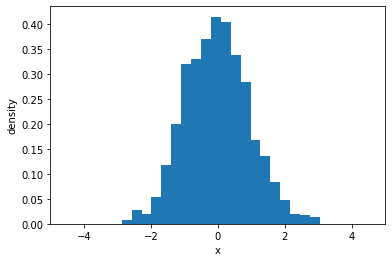
samples = normal.sample(sample_shape=(1000,))
plt.hist(samples, bins=20, density=True)
plt.xlim(-5, 5)
plt.xlabel("x")
plt.ylabel("density")
Text(0, 0.5, 'density')
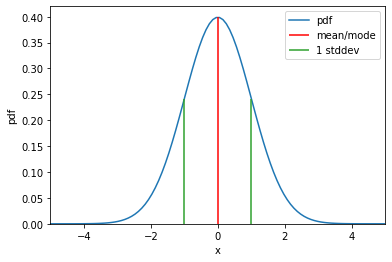
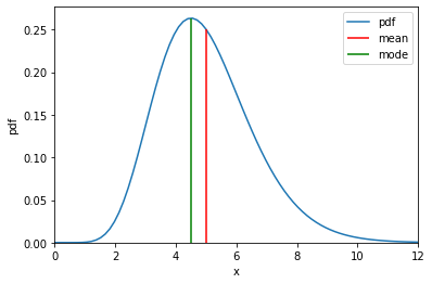
Probability density function
\[\mathrm{Normal}(x \mid \mu, \sigma) = \frac{1}{\sigma \sqrt{2\pi}}\exp \left( {-\frac{(x-\mu)^2}{2 \sigma^2}} \right)\]# Values of x are within support
x = torch.linspace(-5, 5, 100)
# Take exponent of log_prob to get pdf
normal_pdf = normal.log_prob(x).exp()
plt.plot(x, normal_pdf, label="pdf")
# Plot mean and mode
plt.vlines(normal.mean, ymin=0, ymax=normal.log_prob(normal.mean).exp(), colors="r", label="mean/mode")
plt.vlines(normal.scale, ymin=0, ymax=normal.log_prob(normal.scale).exp(), colors="C2", label="1 stddev")
plt.vlines(-normal.scale, ymin=0, ymax=normal.log_prob(normal.scale).exp(), colors="C2")
plt.xlabel("x")
plt.ylabel("pdf")
plt.xlim(-5, 5)
plt.ylim(0, 0.42)
plt.legend()
plt.show()
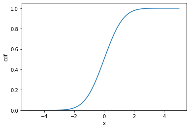
Cumulative density function
normal_cdf = normal.cdf(x)
plt.plot(x, normal_cdf)

plt.xlabel("x")
plt.ylabel("cdf")
plt.ylim(0)
plt.show()
Distribution creation
\(\mathrm{Gamma}(x \mid \alpha, \, \beta)\) \(\alpha \in \mathbb{R}_{\gt 0}\) \(\beta \in \mathbb{R}_{\gt 0}\)
# Gamma distribution is parameterized by concentration (alpha) and rate (beta)
gamma = dist.Gamma(concentration=torch.tensor(10.0), rate=torch.tensor(2.0))
print("gamma = dist.Gamma(concentration=torch.tensor(10.0), rate=torch.tensor(2.0))")
print(f"gamma.concentration = {gamma.concentration}  # alpha")
print(f"gamma.rate = {gamma.rate}            # beta")

# concentration and rate parameters are constrained to be positive-valued
print(f"gamma.arg_constraints['concentration'] = {gamma.arg_constraints['concentration']}")
print(f"gamma.arg_constraints['rate'] = {gamma.arg_constraints['rate']}")

# Gamma distribution supports positive-valued random variables
print(f"gamma.support = {gamma.support}")
gamma = dist.Gamma(concentration=torch.tensor(10.0), rate=torch.tensor(2.0))
gamma.concentration = 10.0  # alpha
gamma.rate = 2.0            # beta
gamma.arg_constraints['concentration'] = GreaterThan(lower_bound=0.0)
gamma.arg_constraints['rate'] = GreaterThan(lower_bound=0.0)
gamma.support = GreaterThanEq(lower_bound=0.0)
Properties
\(\mathrm{mean} = \frac{\alpha}{\beta}\) \(\mathrm{mode} = \frac{\alpha - 1}{\beta}\) \(\mathrm{stddev} = \sqrt{\frac{\alpha}{\beta^2}}\) \(\mathrm{variance} = \frac{\alpha}{\beta^2}\)
# distribution properties
print(f"gamma.mean = {gamma.mean}")
print(f"gamma.mode = {gamma.mode}")
print(f"gamma.stddev = {gamma.stddev}")
print(f"gamma.variance = {gamma.variance}")
gamma.mean = 5.0
gamma.mode = 4.5
gamma.stddev = 1.5811388492584229
gamma.variance = 2.5
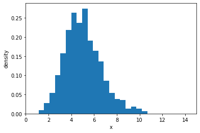
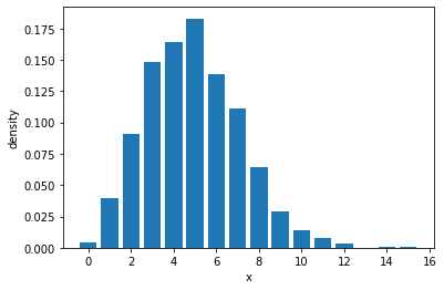
Sampling
\(x \sim \mathrm{Gamma}(\alpha,\,\beta)\) \(x \in \mathbb{R}_{\gt 0}\)
# sample values are within this support
print(f"gamma.support = {gamma.support}")
# run this multiple times - each time you will get different random values
sample = gamma.sample()
print(f"gamma.sample() = {sample}")
gamma.support = GreaterThanEq(lower_bound=0.0)
gamma.sample() = 2.986645460128784
samples = gamma.sample(sample_shape=(1000,))
plt.hist(samples, bins=20, density=True)
plt.xlim(0, 15)
plt.xlabel("x")
plt.ylabel("density")
Text(0, 0.5, 'density')
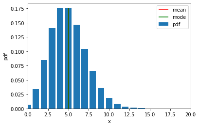
Probability density function
\[\mathrm{Gamma}(x \mid \alpha, \, \beta) = \frac{\beta^\alpha}{\Gamma (\alpha)}x ^{\alpha-1} e^{-\beta x}\]# Define values of x within support
x = torch.linspace(0, 15, 100)
# Take exponent of log_prob to get pdf
gamma_pdf = gamma.log_prob(x).exp()
plt.plot(x, gamma_pdf, label="pdf")
# Plot mean and mode
plt.vlines(gamma.mean, ymin=0, ymax=gamma.log_prob(gamma.mean).exp(), colors="r", label="mean")
plt.vlines(gamma.mode, ymin=0, ymax=gamma.log_prob(gamma.mode).exp(), colors="g", label="mode")
plt.xlabel("x")
plt.ylabel("pdf")
plt.xlim(0, 12)
plt.ylim(0)
plt.legend()
plt.show()
Delta Distribution
Distribution creation
\(\mathrm{Poisson}(x \mid \lambda)\) \(\lambda \in \mathbb{R}_{\gt 0}\)
# Poisson distribution is parameterized by rate (lambda)
poisson = dist.Poisson(rate=torch.tensor(5.0))
print("poisson = dist.Poisson(rate=torch.tensor(5.0))")
print(f"poisson.rate = {poisson.rate}            # lambda")

# rate parameter is constrained to be positive-valued
print(f"poisson.arg_constraints['rate'] = {poisson.arg_constraints['rate']}")

# Poisson distribution supports nonnegative-integer random variables
print(f"poisson.support = {poisson.support}")
poisson = dist.Poisson(rate=torch.tensor(5.0))
poisson.rate = 5.0            # lambda
poisson.arg_constraints['rate'] = GreaterThanEq(lower_bound=0.0)
poisson.support = IntegerGreaterThan(lower_bound=0)
Properties
\(\mathrm{mean} = \lambda\) \(\mathrm{mode} = \lambda\) \(\mathrm{stddev} = \sqrt{\lambda}\) \(\mathrm{variance} = \lambda\)
# distribution properties
print(f"poisson.mean = {poisson.mean}")
print(f"poisson.mode = {poisson.mode}")
print(f"poisson.stddev = {poisson.stddev}")
print(f"poisson.variance = {poisson.variance}")
poisson.mean = 5.0
poisson.mode = 5.0
poisson.stddev = 2.2360680103302
poisson.variance = 5.0
Sampling
\(x \sim \mathrm{Poisson}(\lambda)\) \(x \in \mathbb{Z}_{\ge 0}\)
# sample values are within this support
print(f"poisson.support = {poisson.support}")
# run this multiple times - each time you will get different random values
sample = poisson.sample()
print(f"poisson.sample() = {sample}")
poisson.support = IntegerGreaterThan(lower_bound=0)
poisson.sample() = 5.0
samples = poisson.sample(sample_shape=(1000,))
sample_values, sample_counts = torch.unique(samples, return_counts=True)
plt.bar(sample_values, sample_counts / 1000)
plt.xlabel("x")
plt.ylabel("density")
Text(0, 0.5, 'density')
Probability density function
\[\mathrm{Poisson}(x \mid \lambda) = \lambda^x \frac{e^{-\lambda}}{x!}\]# Define values of x within support
x = torch.arange(0, 20)
# Take exponent of log_prob to get pdf
poisson_pdf = poisson.log_prob(x).exp()
plt.bar(x, poisson_pdf, label="pdf")
# Plot mean and mode
plt.vlines(poisson.mean, ymin=0, ymax=poisson.log_prob(poisson.mean).exp(), colors="r", label="mean")
plt.vlines(poisson.mode, ymin=0, ymax=poisson.log_prob(poisson.mode).exp(), colors="g", label="mode")
plt.xlabel("x")
plt.ylabel("pdf")
plt.xlim(0, 20)
plt.ylim(0)
plt.legend()
plt.show()
# NumPy routines which allocate memory and fill arrays with value
try:
    bernoulli = dist.Bernoulli(probs=0.3, logits=0)
except Exception as e:
    print("The error message you'll see is:")
    print(e)
The error message you'll see is:
Either `probs` or `logits` must be specified, but not both.
Distribution creation
\(\mathrm{Bernoulli}(x \mid p)\) \(p \in [0, 1]\)
or alternatively by logit(p)
\(\mathrm{Bernoulli}(x \mid \mathrm{logit}(p))\) where \(\mathrm{logit}(p) = \log \frac{p}{1-p}\)
# Bernoulli distribution is parameterized by probs (p)
bernoulli_probs = dist.Bernoulli(probs=torch.tensor(0.3))
print("bernoulli_probs = dist.Bernoulli(probs=torch.tensor(0.3))")
print(f"bernoulli_probs.probs = {bernoulli_probs.probs}            # p")
print(f"bernoulli_probs.logits = {bernoulli_probs.logits}            # logit(p)")

# Verify logit(p)
print(f"logit(p) = {torch.log(bernoulli_probs.probs / (1 - bernoulli_probs.probs))}")

# rate parameter is constrained to be positive-valued
print(f"bernoulli_probs.arg_constraints['probs'] = {bernoulli_probs.arg_constraints['probs']}")
print(f"bernoulli_probs.arg_constraints['logits'] = {bernoulli_probs.arg_constraints['logits']}")

# Bernoulli distribution supports binary random variables
print(f"bernoulli_probs.support = {bernoulli_probs.support}")
bernoulli_probs = dist.Bernoulli(probs=torch.tensor(0.3))
bernoulli_probs.probs = 0.30000001192092896            # p
bernoulli_probs.logits = -0.8472978472709656            # logit(p)
logit(p) = -0.8472977876663208
bernoulli_probs.arg_constraints['probs'] = Interval(lower_bound=0.0, upper_bound=1.0)
bernoulli_probs.arg_constraints['logits'] = Real()
bernoulli_probs.support = Boolean()
# Bernoulli distribution is parameterized by probs (p)
bernoulli_logits = dist.Bernoulli(logits=torch.tensor(0.0))
print("bernoulli_logits = dist.Bernoulli(probs=torch.tensor(0.3))")
print(f"bernoulli_logits.probs = {bernoulli_logits.probs}            # p")
print(f"bernoulli_logits.logits = {bernoulli_logits.logits}            # logit(p)")

# Verify inverse of logit(p)
print(f"p = {1 / (1 + torch.exp(-bernoulli_logits.logits))}")

# rate parameter is constrained to be positive-valued
print(f"bernoulli_logits.arg_constraints['probs'] = {bernoulli_logits.arg_constraints['probs']}")
print(f"bernoulli_logits.arg_constraints['logits'] = {bernoulli_logits.arg_constraints['logits']}")

# Bernoulli distribution supports binary random variables
print(f"bernoulli_logits.support = {bernoulli_logits.support}")
bernoulli_logits = dist.Bernoulli(probs=torch.tensor(0.3))
bernoulli_logits.probs = 0.5            # p
bernoulli_logits.logits = 0.0            # logit(p)
p = 0.5
bernoulli_logits.arg_constraints['probs'] = Interval(lower_bound=0.0, upper_bound=1.0)
bernoulli_logits.arg_constraints['logits'] = Real()
bernoulli_logits.support = Boolean()
Properties
\(\mathrm{mean} = p\) \begin{align} \mathrm{mode} = \left{ \begin{array}{cl} 0 & p \lt 0.5
1 & p > 0.5 \end{array} \right. \end{align} \(\mathrm{stddev} = \sqrt{p(1-p)}\) \(\mathrm{variance} = p(1-p)\)
# distribution properties
print(f"bernoulli_probs.mean = {bernoulli_probs.mean}")
print(f"bernoulli_probs.mode = {bernoulli_probs.mode}")
print(f"bernoulli_probs.stddev = {bernoulli_probs.stddev}")
print(f"bernoulli_probs.variance = {bernoulli_probs.variance}")
bernoulli_probs.mean = 0.30000001192092896
bernoulli_probs.mode = 0.0
bernoulli_probs.stddev = 0.4582575857639313
bernoulli_probs.variance = 0.21000000834465027
Sampling
\(x \sim \mathrm{Bernoulli}(p)\) \(x \in \{0, \, 1 \}\)
# sample values are within this support
print(f"bernoulli_probs.support = {bernoulli_probs.support}")
# run this multiple times - each time you will get different random values
sample = bernoulli_probs.sample()
print(f"bernoulli_probs.sample() = {sample}")
bernoulli_probs.support = Boolean()
bernoulli_probs.sample() = 1.0
samples = bernoulli_probs.sample(sample_shape=(1000,))
sample_values, sample_counts = torch.unique(samples, return_counts=True)
plt.bar(sample_values, sample_counts / 1000)
plt.xlabel("x")
plt.ylabel("density")
Text(0, 0.5, 'density')
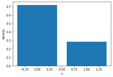
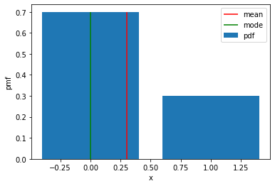
Probability density function
\[\mathrm{Bernoulli}(x \mid p) = p^{x} (1-p)^{1-x}\]# Define values of x within support
x = torch.tensor([0.0, 1.0])
# Take exponent of log_prob to get pdf
bernoulli_pdf = bernoulli_probs.log_prob(x).exp()
plt.bar(x, bernoulli_pdf, label="pdf")
# Plot mean and mode
plt.vlines(bernoulli_probs.mean, ymin=0, ymax=0.7, colors="r", label="mean")
plt.vlines(bernoulli_probs.mode, ymin=0, ymax=0.7, colors="g", label="mode")
plt.xlabel("x")
plt.ylabel("pmf")
# plt.xlim(0, 20)
plt.ylim(0)
plt.legend()
plt.show()
categorical_probs = dist.Categorical(probs=torch.tensor([0.3, 0.5, 0.1, 0.1]))
print(f"categorical_probs = {categorical_probs}")
print(f"support = {categorical_probs.support}  # sample values are within this support")
print("Distribution parameters:")
print(f"probs: value = {categorical_probs.probs}, constraint = {categorical_probs.arg_constraints['probs']}")
print(f"logits: value = {categorical_probs.logits}, constraint = {categorical_probs.arg_constraints['logits']}")
print("Distribution properties:")
print(f"mean = {categorical_probs.mean}               # equals to rate")
print(f"mode = {categorical_probs.mode}               # equals to rate")
print(f"standard deviation = {categorical_probs.stddev} # equals to sqrt(rate)")
print(f"variance = {categorical_probs.variance}           # equals to rate")
categorical_probs = Categorical(probs: torch.Size([4]))
support = IntegerInterval(lower_bound=0, upper_bound=3)  # sample values are within this support
Distribution parameters:
probs: value = tensor([0.3000, 0.5000, 0.1000, 0.1000]), constraint = Simplex()
logits: value = tensor([-1.2040, -0.6931, -2.3026, -2.3026]), constraint = IndependentConstraint(Real(), 1)
Distribution properties:
mean = nan               # equals to rate
mode = 1               # equals to rate
standard deviation = nan # equals to sqrt(rate)
variance = nan           # equals to rate
categorical_probs = dist.Categorical(probs=torch.tensor([0.5, 1, 0.7, 0.3]))
print(f"categorical_probs = {categorical_probs}")
print(f"support = {categorical_probs.support}  # sample values are within this support")
print("Distribution parameters:")
print(f"probs: value = {categorical_probs.probs}, constraint = {categorical_probs.arg_constraints['probs']}")
print(f"logits: value = {categorical_probs.logits}, constraint = {categorical_probs.arg_constraints['logits']}")
print("Distribution properties:")
print(f"mean = {categorical_probs.mean}               # equals to rate")
print(f"mode = {categorical_probs.mode}               # equals to rate")
print(f"standard deviation = {categorical_probs.stddev} # equals to sqrt(rate)")
print(f"variance = {categorical_probs.variance}           # equals to rate")
categorical_probs = Categorical(probs: torch.Size([4]))
support = IntegerInterval(lower_bound=0, upper_bound=3)  # sample values are within this support
Distribution parameters:
probs: value = tensor([0.2000, 0.4000, 0.2800, 0.1200]), constraint = Simplex()
logits: value = tensor([-1.6094, -0.9163, -1.2730, -2.1203]), constraint = IndependentConstraint(Real(), 1)
Distribution properties:
mean = nan               # equals to rate
mode = 1               # equals to rate
standard deviation = nan # equals to sqrt(rate)
variance = nan           # equals to rate
categorical_logits = dist.Categorical(logits=torch.tensor([0.5, 1, -1, 0]))
print(f"categorical_logits = {categorical_logits}")
print(f"support = {categorical_logits.support}  # sample values are within this support")
print("Distribution parameters:")
print(f"probs: value = {categorical_logits.probs}, constraint = {categorical_logits.arg_constraints['probs']}")
print(f"logits: value = {categorical_logits.logits}, constraint = {categorical_logits.arg_constraints['logits']}")
print("Distribution properties:")
print(f"mean = {categorical_logits.mean}               # equals to rate")
print(f"mode = {categorical_logits.mode}               # equals to rate")
print(f"standard deviation = {categorical_logits.stddev} # equals to sqrt(rate)")
print(f"variance = {categorical_logits.variance}           # equals to rate")
categorical_logits = Categorical(logits: torch.Size([4]))
support = IntegerInterval(lower_bound=0, upper_bound=3)  # sample values are within this support
Distribution parameters:
probs: value = tensor([0.2875, 0.4740, 0.0641, 0.1744]), constraint = Simplex()
logits: value = tensor([-1.2466, -0.7466, -2.7466, -1.7466]), constraint = IndependentConstraint(Real(), 1)
Distribution properties:
mean = nan               # equals to rate
mode = 1               # equals to rate
standard deviation = nan # equals to sqrt(rate)
variance = nan           # equals to rate
Some data creation routines do not take a shape tuple:
# NumPy routines which allocate memory and fill arrays with value but do not accept shape as input argument
a = np.arange(4.);              print(f"np.arange(4.):     a = {a}, a shape = {a.shape}, a data type = {a.dtype}")
a = np.random.rand(4);          print(f"np.random.rand(4): a = {a}, a shape = {a.shape}, a data type = {a.dtype}")
values can be specified manually as well.
# NumPy routines which allocate memory and fill with user specified values
a = np.array([5,4,3,2]);  print(f"np.array([5,4,3,2]):  a = {a},     a shape = {a.shape}, a data type = {a.dtype}")
a = np.array([5.,4,3,2]); print(f"np.array([5.,4,3,2]): a = {a}, a shape = {a.shape}, a data type = {a.dtype}")
These have all created a one-dimensional vector a with four elements. a.shape returns the dimensions. Here we see a.shape = (4,) indicating a 1-d array with 4 elements.
3.4 Operations on Distributions
Let’s explore some operations using vectors.
3.4.1 Sampling
Elements of vectors can be accessed via indexing and slicing. NumPy provides a very complete set of indexing and slicing capabilities. We will explore only the basics needed for the course here. Reference Slicing and Indexing for more details.
Indexing means referring to an element of an array by its position within the array.
Slicing means getting a subset of elements from an array based on their indices.
NumPy starts indexing at zero so the 3rd element of an vector $\mathbf{a}$ is a[2].
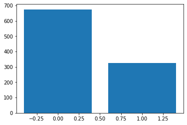
print(f"support = {bernoulli_probs.support}  # sample values are within this support")
sample = bernoulli_probs.sample()
print(f"sample ~ gamma: value = {sample} # run this multiple times - each time you will get different random values")
support = Boolean()  # sample values are within this support
sample ~ gamma: value = 0.0 # run this multiple times - each time you will get different random values
samples = bernoulli_probs.sample(sample_shape=(1000,))
sample_values, sample_counts = torch.unique(samples, return_counts=True)
plt.bar(sample_values, sample_counts)
<BarContainer object of 2 artists>
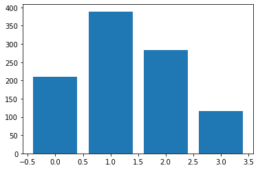
print(f"support = {categorical_probs.support}  # sample values are within this support")
sample = categorical_probs.sample()
print(f"sample ~ categorical: value = {sample} # run this multiple times - each time you will get different random values")
support = IntegerInterval(lower_bound=0, upper_bound=3)  # sample values are within this support
sample ~ categorical: value = 1 # run this multiple times - each time you will get different random values
samples = categorical_probs.sample(sample_shape=(1000,))
sample_values, sample_counts = torch.unique(samples, return_counts=True)
plt.bar(sample_values, sample_counts)
<BarContainer object of 4 artists>
#vector indexing operations on 1-D vectors
a = np.arange(10)
print(a)

#access an element
print(f"a[2].shape: {a[2].shape} a[2]  = {a[2]}, Accessing an element returns a scalar")

# access the last element, negative indexes count from the end
print(f"a[-1] = {a[-1]}")

#indexs must be within the range of the vector or they will produce and error
try:
    c = a[10]
except Exception as e:
    print("The error message you'll see is:")
    print(e)
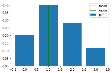
3.4.2 Log-probability
Slicing creates an array of indices using a set of three values (start:stop:step). A subset of values is also valid. Its use is best explained by example:
categorical_probs.support.lower_bound
0
x_min = categorical_probs.support.lower_bound
x_max = categorical_probs.support.upper_bound
x = torch.arange(x_min, x_max + 1)
categorical_pdf = categorical_probs.log_prob(x).exp()
plt.bar(x, categorical_pdf, label="pdf")
plt.vlines(categorical_probs.mean, ymin=0, ymax=0.4, colors="r", label="mean")
plt.vlines(categorical_probs.mode, ymin=0, ymax=0.4, colors="g", label="mode")
# plt.xlim(0, 20)
plt.ylim(0)
plt.legend()
plt.show()
/usr/local/lib/python3.9/dist-packages/matplotlib/axes/_base.py:2503: UserWarning: Warning: converting a masked element to nan.
  xys = np.asarray(xys)
#vector slicing operations
a = np.arange(10)
print(f"a         = {a}")

#access 5 consecutive elements (start:stop:step)
c = a[2:7:1];     print("a[2:7:1] = ", c)

# access 3 elements separated by two
c = a[2:7:2];     print("a[2:7:2] = ", c)

# access all elements index 3 and above
c = a[3:];        print("a[3:]    = ", c)

# access all elements below index 3
c = a[:3];        print("a[:3]    = ", c)

# access all elements
c = a[:];         print("a[:]     = ", c)
3.4.3 Single vector operations
There are a number of useful operations that involve operations on a single vector.
a = np.array([1,2,3,4])
print(f"a             : {a}")
# negate elements of a
b = -a
print(f"b = -a        : {b}")

# sum all elements of a, returns a scalar
b = np.sum(a)
print(f"b = np.sum(a) : {b}")

b = np.mean(a)
print(f"b = np.mean(a): {b}")

b = a**2
print(f"b = a**2      : {b}")
3.4.4 Vector Vector element-wise operations
Most of the NumPy arithmetic, logical and comparison operations apply to vectors as well. These operators work on an element-by-element basis. For example \(c_i = a_i + b_i\)
a = np.array([ 1, 2, 3, 4])
b = np.array([-1,-2, 3, 4])
print(f"Binary operators work element wise: {a + b}")
Of course, for this to work correctly, the vectors must be of the same size:
#try a mismatched vector operation
c = np.array([1, 2])
try:
    d = a + c
except Exception as e:
    print("The error message you'll see is:")
    print(e)
3.4.5 Scalar Vector operations
Vectors can be ‘scaled’ by scalar values. A scalar value is just a number. The scalar multiplies all the elements of the vector.
a = np.array([1, 2, 3, 4])

# multiply a by a scalar
b = 5 * a
print(f"b = 5 * a : {b}")
3.4.6 Vector Vector dot product
The dot product is a mainstay of Linear Algebra and NumPy. This is an operation used extensively in this course and should be well understood. The dot product is shown below.
![]()
The dot product multiplies the values in two vectors element-wise and then sums the result. Vector dot product requires the dimensions of the two vectors to be the same.
Let’s implement our own version of the dot product below:
Using a for loop, implement a function which returns the dot product of two vectors. The function to return given inputs $a$ and $b$: \(x = \sum_{i=0}^{n-1} a_i b_i\) Assume both a and b are the same shape.
def my_dot(a, b):
    """
   Compute the dot product of two vectors

    Args:
      a (ndarray (n,)):  input vector
      b (ndarray (n,)):  input vector with same dimension as a

    Returns:
      x (scalar):
    """
    x=0
    for i in range(a.shape[0]):
        x = x + a[i] * b[i]
    return x
# test 1-D
a = np.array([1, 2, 3, 4])
b = np.array([-1, 4, 3, 2])
print(f"my_dot(a, b) = {my_dot(a, b)}")
Note, the dot product is expected to return a scalar value.
Let’s try the same operations using np.dot.
# test 1-D
a = np.array([1, 2, 3, 4])
b = np.array([-1, 4, 3, 2])
c = np.dot(a, b)
print(f"NumPy 1-D np.dot(a, b) = {c}, np.dot(a, b).shape = {c.shape} ")
c = np.dot(b, a)
print(f"NumPy 1-D np.dot(b, a) = {c}, np.dot(a, b).shape = {c.shape} ")
Above, you will note that the results for 1-D matched our implementation.
3.4.7 The Need for Speed: vector vs for loop
We utilized the NumPy library because it improves speed memory efficiency. Let’s demonstrate:
np.random.seed(1)
a = np.random.rand(10000000)  # very large arrays
b = np.random.rand(10000000)

tic = time.time()  # capture start time
c = np.dot(a, b)
toc = time.time()  # capture end time

print(f"np.dot(a, b) =  {c:.4f}")
print(f"Vectorized version duration: {1000*(toc-tic):.4f} ms ")

tic = time.time()  # capture start time
c = my_dot(a,b)
toc = time.time()  # capture end time

print(f"my_dot(a, b) =  {c:.4f}")
print(f"loop version duration: {1000*(toc-tic):.4f} ms ")

del(a);del(b)  #remove these big arrays from memory
So, vectorization provides a large speed up in this example. This is because NumPy makes better use of available data parallelism in the underlying hardware. GPU’s and modern CPU’s implement Single Instruction, Multiple Data (SIMD) pipelines allowing multiple operations to be issued in parallel. This is critical in Machine Learning where the data sets are often very large.
3.4.8 Vector Vector operations in Course 1
Vector Vector operations will appear frequently in course 1. Here is why:
- Going forward, our examples will be stored in an array,
X_trainof dimension (m,n). This will be explained more in context, but here it is important to note it is a 2 Dimensional array or matrix (see next section on matrices). wwill be a 1-dimensional vector of shape (n,).- we will perform operations by looping through the examples, extracting each example to work on individually by indexing X. For example:
X[i] X[i]returns a value of shape (n,), a 1-dimensional vector. Consequently, operations involvingX[i]are often vector-vector.
That is a somewhat lengthy explanation, but aligning and understanding the shapes of your operands is important when performing vector operations.
# show common Course 1 example
X = np.array([[1],[2],[3],[4]])
w = np.array([2])
c = np.dot(X[1], w)

print(f"X[1] has shape {X[1].shape}")
print(f"w has shape {w.shape}")
print(f"c has shape {c.shape}")
4 Matrices
4.1 Abstract
Matrices, are two dimensional arrays. The elements of a matrix are all of the same type. In notation, matrices are denoted with capitol, bold letter such as $\mathbf{X}$. In this and other labs, m is often the number of rows and n the number of columns. The elements of a matrix can be referenced with a two dimensional index. In math settings, numbers in the index typically run from 1 to n. In computer science and these labs, indexing will run from 0 to n-1.
